10 Minutes to Pandas Python Tutorial

Introduction

Data is everywhere, and handling data efficiently is crucial for anyone working in data science, analytics, or even simple data processing tasks. This is where Pandas, a powerful Python library, comes into play. Let’s explore 10 Minutes to Pandas.

Pandas makes it easy to organize, clean, manipulate, and analyse data effortlessly. Whether you’re dealing with Excel files, CSVs, databases, or raw data from APIs (JSON, XML), Pandas provides intuitive tools to transform messy data into meaningful insights.

In this guide, you will learn:

• How to install and setup Pandas
• Working with Series and DataFrame (the core data structures)
• Loading data from different sources
• Cleaning and manipulating data efficiently
• Analysing data using grouping, sorting, and filtering
• Merging and joining datasets
• Performing time series analysis
• Visualizing data directly with Pandas

By the end of this guide, you’ll be able to handle real-world datasets efficiently and apply Pandas to various scenarios. Let’s dive in!

What is Pandas in 10 Minutes?

Pandas, a versatile tool, excels at data manipulation and analysis. It serves as a data haven, enabling data cleansing, transformation, and exploration.

Consider a CSV dataset: Pandas effortlessly converts it into a DataFrame, a structured table. From here, a world of possibilities awaits:

• Compute Statistics: Uncover insights by calculating averages, medians, maximums, minimums, or correlations between columns.
• Data Cleansing: Addressing data inconsistencies by removing missing values and filtering rows or columns based on specified criteria.
• Visualization: Leveraging Matplotlib’s capabilities, collaboratively visualize data, creating bars, lines, histograms, and other graphical representations.
• Persistence: Effortlessly store refined data back into a CSV, another file format, or a database for easy access.

In essence, Pandas serves as a bridge for seamless data navigation, providing a comprehensive suite of functionalities for efficient data management. You can learn Python built-ins function in other article.

The Cornerstone of Data Manipulation and Analysis (10 Minutes to Pandas)

The fundamental building block of Pandas is its DataFrame, which provides a well-structured platform to explore and manipulate data, converting the initial raw data to a more structured format. This hierarchical design allows for smooth interoperability with other popular libraries like NumPy, Matplotlib, and scikit-learn, enabling data scientists to easily move from raw data to actionable insights.

Pandas is powerful, evidenced by its vast array of features, spanning from data cleansing and statistical analysis to data visualization. From removing inconsistencies, applying patterns, or computing statistical arrays, Pandas helps ensure a seamless trajectory from data ingestion to insight.

Key Highlights in 10 Minutes to Pandas

• Data Cleansing: Clean the data by eliminating missing values, outliers, and inconsistencies, maintaining the data integrity.
• Statistical Analysis: Calculate descriptive stats, run hypothesis tests or discover correlations to learn more about the data.
• Data Visualization: Develop the visualizations (e.g., bar charts, line graphs, histograms, scatter plots, etc.) to the insights and communicate those effectively.

10 Minues to Pandas in Data Science Companion

Pandas’ unwavering commitment to efficiency, versatility, and interoperability has cemented its position as an indispensable tool for data scientists. Its ability to transform raw data into actionable insights makes it an essential component of the data science toolkit, empowering data scientists to tackle complex challenges and derive meaningful conclusions from vast datasets.

Getting Started with 10 Minutes to Pandas Python Tutorial

Installation of Pandas in 10 Minutes

Let’s start the Pandas Python Tutorial from begining. Ensure the Pandas library is installed within your Python environment. If not, use the following command:

Using pip:

pip install pandas

pip install pandas

Using conda

conda install pandas

conda install pandas

!pip install pandas

Importing Pandas

Once installed, import Pandas in your script using the standard convention:

import pandas as pd

The alias pd is commonly used to keep the code concise.

Pandas Data Structures in 10 Minutes

Python Pandas has two primary data structures:

1. Series – A one-dimensional labelled array (like a list or dictionary).
2. DataFrame – A two-dimensional labelled table (like an Excel sheet or database table).

Pandas Series

A Series in Pandas is a one-dimensional array that holds data along with an index. You can think of a Series as a single column in a spreadsheet. It’s a one-dimensional labelled array. Each piece of data has an “index” (like a row number or a name) that helps you find it.

A Series could represent:

• A list of daily temperatures.
• A column of customer ages.
• A list of stock prices for one company.

Creating a Pandas Series

Let’s assume you have a list of fruit prices:

import pandas as pd

index = ['Apple', 'Mango', 'Banana', 'Grapes']

data = [100, 200, 300, 400]

prices = pd.Series(data=data, index=index)

print(prices)

import pandas as pd

index = ['Apple', 'Mango', 'Banana', 'Grapes']

data = [100, 200, 300, 400]

prices = pd.Series(data=data, index=index)

print(prices)

Output:

Apple     100
Mango     200
Banana    300
Grapes    400
dtype: int64

Real Example – Daily Stock Prices

Let’s create a Series to represent daily stock prices for Tata Motors:

prices = pd.Series([450, 460, 455, 470, 475], index=['Monday', 'Tuesday', 'Wednesday', 'Thursday', 'Friday'])

print(prices)

prices = pd.Series([450, 460, 455, 470, 475], index=['Monday', 'Tuesday', 'Wednesday', 'Thursday', 'Friday'])

print(prices)

Output:
Monday       450
Tuesday      460
Wednesday    455
Thursday     470
Friday       475
dtype: int64

Accessing Elements in a Series

You can access elements of pandas series using index labels:

print(prices['Monday'])

print(prices['Monday'])

Output: 
450

Pandas DataFrame

The cornerstone of Pandas, a DataFrame is a tabular data structure consisting of rows and columns. We can create a DataFrame from various sources like lists, dictionaries, CSV files, or NumPy arrays.

A DataFrame is simply a two-dimensional data structure similar to an Excel spreadsheet.

• A DataFrame is like a whole spreadsheet – rows and columns. It’s a two-dimensional labelled data structure.
• Rows and Columns: It has rows (like individual records) and columns (like different attributes of those records).
• Example: Let’s create a sample DataFrame using Pandas.

Creating a DataFrame in Pandas

Let’s create a DataFrame with employee_name, phone_number, city, and date_of_birth:

import pandas as pd

# Create a DataFrame with employee details
data = {
'employee_id': [101, 102, 103, 104, 105, 106, 107, 108, 109, 110],
'employee_name': ['Aarav Sharma', 'Vivaan Patel', 'Aditya Nair', 
                  'Vihaan Reddy', 'Arjun Singh', 'Sai Kumar', 
                   'Reyansh Gupta', 'Ayaan Joshi', 'Krishna Das', 'Ishaan Mehta'],
'phone_number': ['+91-9876543210', '+91-8765432109', '+91-7654321098', 
                 '+91-6543210987', '+91-5432109876', '+91-4321098765', 
                 '+91-3210987654', '+91-2109876543', '+91-1098765432', 
                 '+91-0987654321'],
'city': ['Mumbai', 'Delhi', 'Bengaluru', 'Hyderabad', 'Chennai',
             'Kolkata', 'Pune', 'Ahmedabad', 'Jaipur', 'Surat'],
'date_of_birth': ['1990-01-15', '1992-03-22', '1988-05-30', '1995-07-19', 
                '1991-09-10', '1993-11-25', '1989-12-05', '1994-02-14', 
               '1990-06-18', '1992-08-29']
}

df = pd.DataFrame(data)

print(df)

import pandas as pd

# Create a DataFrame with employee details
data = {
'employee_id': [101, 102, 103, 104, 105, 106, 107, 108, 109, 110],
'employee_name': ['Aarav Sharma', 'Vivaan Patel', 'Aditya Nair', 
                  'Vihaan Reddy', 'Arjun Singh', 'Sai Kumar', 
                   'Reyansh Gupta', 'Ayaan Joshi', 'Krishna Das', 'Ishaan Mehta'],
'phone_number': ['+91-9876543210', '+91-8765432109', '+91-7654321098', 
                 '+91-6543210987', '+91-5432109876', '+91-4321098765', 
                 '+91-3210987654', '+91-2109876543', '+91-1098765432', 
                 '+91-0987654321'],
'city': ['Mumbai', 'Delhi', 'Bengaluru', 'Hyderabad', 'Chennai',
             'Kolkata', 'Pune', 'Ahmedabad', 'Jaipur', 'Surat'],
'date_of_birth': ['1990-01-15', '1992-03-22', '1988-05-30', '1995-07-19', 
                '1991-09-10', '1993-11-25', '1989-12-05', '1994-02-14', 
               '1990-06-18', '1992-08-29']
}

df = pd.DataFrame(data)

print(df)

   employee_id  employee_name    phone_number       city date_of_birth
0          101   Aarav Sharma  +91-9876543210     Mumbai    1990-01-15
1          102   Vivaan Patel  +91-8765432109      Delhi    1992-03-22
2          103    Aditya Nair  +91-7654321098  Bengaluru    1988-05-30
3          104   Vihaan Reddy  +91-6543210987  Hyderabad    1995-07-19
4          105    Arjun Singh  +91-5432109876    Chennai    1991-09-10
5          106      Sai Kumar  +91-4321098765    Kolkata    1993-11-25
6          107  Reyansh Gupta  +91-3210987654       Pune    1989-12-05
7          108    Ayaan Joshi  +91-2109876543  Ahmedabad    1994-02-14
8          109    Krishna Das  +91-1098765432     Jaipur    1990-06-18
9          110   Ishaan Mehta  +91-0987654321      Surat    1992-08-29

Print Pandas Dataframe as Table

We can use the to_string() method to print pandas dataframe as table. As this method returns a string representation of the DataFrame in a tabular format. We can then print the string using the print() function.

print(df.to_string())

#Output of print pandas dataframe as table:

   employee_id  employee_name    phone_number       city date_of_birth
0          101   Aarav Sharma  +91-9876543210     Mumbai    1990-01-15
1          102   Vivaan Patel  +91-8765432109      Delhi    1992-03-22
2          103    Aditya Nair  +91-7654321098  Bengaluru    1988-05-30
3          104   Vihaan Reddy  +91-6543210987  Hyderabad    1995-07-19
4          105    Arjun Singh  +91-5432109876    Chennai    1991-09-10
5          106      Sai Kumar  +91-4321098765    Kolkata    1993-11-25
6          107  Reyansh Gupta  +91-3210987654       Pune    1989-12-05
7          108    Ayaan Joshi  +91-2109876543  Ahmedabad    1994-02-14
8          109    Krishna Das  +91-1098765432     Jaipur    1990-06-18
9          110   Ishaan Mehta  +91-0987654321      Surat    1992-08-29

print(df.to_string())

#Output of print pandas dataframe as table:

   employee_id  employee_name    phone_number       city date_of_birth
0          101   Aarav Sharma  +91-9876543210     Mumbai    1990-01-15
1          102   Vivaan Patel  +91-8765432109      Delhi    1992-03-22
2          103    Aditya Nair  +91-7654321098  Bengaluru    1988-05-30
3          104   Vihaan Reddy  +91-6543210987  Hyderabad    1995-07-19
4          105    Arjun Singh  +91-5432109876    Chennai    1991-09-10
5          106      Sai Kumar  +91-4321098765    Kolkata    1993-11-25
6          107  Reyansh Gupta  +91-3210987654       Pune    1989-12-05
7          108    Ayaan Joshi  +91-2109876543  Ahmedabad    1994-02-14
8          109    Krishna Das  +91-1098765432     Jaipur    1990-06-18
9          110   Ishaan Mehta  +91-0987654321      Surat    1992-08-29

Add a Row to a Dataframe Pandas

Using Pandas Dataframe.loc

We can add a new row in the existing Pandas Dataframe using dataframe.loc attribute. Since Dataframe.loc is used to get the nth row’s data as pandas series type. We need to create the new row as pandas series and add the row as the last row of the dataframe like below:

data  = {'Name': 'David', 'Age': 27, 'Occupation': 'Data Engineer'} 
index = ['Name', 'Age', 'Occupation']
new_row = pd.Series(data=data, index=index)

last_position = len(df)
df.loc[last_position]=new_row

df

data  = {'Name': 'David', 'Age': 27, 'Occupation': 'Data Engineer'} 
index = ['Name', 'Age', 'Occupation']
new_row = pd.Series(data=data, index=index)

last_position = len(df)
df.loc[last_position]=new_row

df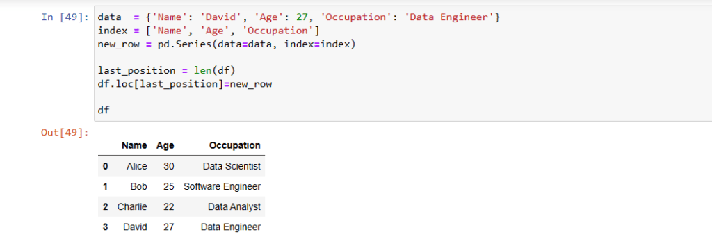

Concatenating Two Dataframes in Pandas (pandas.concat)

You can concatenate two dataframes into a dataframe in Pandas. You can create a new pandas dataframe of one row. Now you can use the pandas.concat method to add the new one row dataframe to the existing dataframe.

new_row=pd.Series(data={'Name': 'David', 'Age': 27, 
                   'Occupation': 'Data Engineer'}, 
                   index=['Name', 'Age','Occupation']
                   )
df2=pd.DataFrame([new_row])
pd.concat([df, df2], ignore_index=True)                   

new_row=pd.Series(data={'Name': 'David', 'Age': 27, 
                   'Occupation': 'Data Engineer'}, 
                   index=['Name', 'Age','Occupation']
                   )
df2=pd.DataFrame([new_row])
pd.concat([df, df2], ignore_index=True)                   

Add Row to Empty Dataframe in Pandas

You can add row into a empty dataframe in Pandas. To add row to empty dataframe you can use the pandas concat method as describe below

import pandas as pd

df = pd.DataFrame()

new_row = pd.DataFrame({'Name': ['David'], 'Age': [28], 'Occupation': ['Data Engineer']})

df = pd.concat([df, new_row], ignore_index=True)

print(df)

import pandas as pd

df = pd.DataFrame()

new_row = pd.DataFrame({'Name': ['David'], 'Age': [28], 'Occupation': ['Data Engineer']})

df = pd.concat([df, new_row], ignore_index=True)

print(df)

Attributeerror: ‘dataframe’ object has no attribute ‘append’

The AttributeError: ‘DataFrame’ object has no attribute ‘append’ error arises when you attempt to utilize the append method on a Pandas DataFrame object. This error stems from the absence of a built-in append method in Pandas DataFrames for directly appending rows. Please use any of the above mentioned method to resolve this. This is how you can add a row to pandas dataframe easily and effectivly.

How to Subtract Two DataFrames in Pandas?

You can use the DataFrame.subtract method to Subtract Two DataFrames. This method performs an element-wise subtraction of the two DataFrames. We can subtract two dataframes in Pandas element by element using this method.

import pandas as pd

# Create two DataFrames
df1 = pd.DataFrame({'a': [1, 2, 3], 'b': [4, 5, 6]})
df2 = pd.DataFrame({'a': [7, 8, 9], 'b': [10, 11, 12]})

# Subtract the two DataFrames using the DataFrame.subtract() method
df_sub = df1.subtract(df2)

# Print the result
print(df_sub) 

# Output of pandas subtract two dataframes

   a  b
0 -6 -6
1 -6 -6
2 -6 -6

import pandas as pd

# Create two DataFrames
df1 = pd.DataFrame({'a': [1, 2, 3], 'b': [4, 5, 6]})
df2 = pd.DataFrame({'a': [7, 8, 9], 'b': [10, 11, 12]})

# Subtract the two DataFrames using the DataFrame.subtract() method
df_sub = df1.subtract(df2)

# Print the result
print(df_sub) 

# Output of pandas subtract two dataframes

   a  b
0 -6 -6
1 -6 -6
2 -6 -6

How to Slice a DataFrame in Pandas?

You can use the DataFrame.iloc method to slice pandas dataframe. This method allows you to slice the DataFrame using integer indices. The indices can be specified individually or as a range.

import pandas as pd

#Create a DataFrame
df = pd.DataFrame({'a': [1, 2, 3, 4, 5], 'b': [6, 7, 8, 9, 10]})

#pandas dataframe slicing using the DataFrame.iloc() method
df_sliced = df.iloc[:3, :]

# Print the sliced DataFrame
print(df_sliced)


OUTPUT:

   a  b
0  1  6
1  2  7
2  3  8

import pandas as pd

#Create a DataFrame
df = pd.DataFrame({'a': [1, 2, 3, 4, 5], 'b': [6, 7, 8, 9, 10]})

#pandas dataframe slicing using the DataFrame.iloc() method
df_sliced = df.iloc[:3, :]

# Print the sliced DataFrame
print(df_sliced)


OUTPUT:

   a  b
0  1  6
1  2  7
2  3  8

Convert Pandas to Spark Dataframe: 10 Minutes to Pandas

We can convert pandas dataframe to pyspark dataframe, we can use the following steps:

• Create a SparkSession object.
• Import the Pandas DataFrame.
• Use the createDataFrame() method to convert the Pandas DataFrame to a Spark DataFrame.
• Define the schema for the Spark DataFrame (optional).
• Save the Spark DataFrame to a file or cache it in memory.
  Here is an example of how to convert a Pandas DataFrame to a Spark DataFrame using the Python API:

from pyspark.sql import SparkSession

#Create PySpark Season
spark = SparkSession.builder.appName("PandasDf2SparkDf").getOrCreate()

#Enable Apache Arrow to convert Pandas to PySpark DataFrame
spark.conf.set("spark.sql.execution.arrow.enabled", "true")

spark_df = spark.createDataFrame(df)

spark_df.show(5)

from pyspark.sql import SparkSession

#Create PySpark Season
spark = SparkSession.builder.appName("PandasDf2SparkDf").getOrCreate()

#Enable Apache Arrow to convert Pandas to PySpark DataFrame
spark.conf.set("spark.sql.execution.arrow.enabled", "true")

spark_df = spark.createDataFrame(df)

spark_df.show(5)

Convert List to Pandas Dataframe: 10 Minutes

We can convert a list to a Pandas DataFrame using the pd.DataFrame() constructor in Pandas. Here’s an example:

Let’s assume you have a list of lists containing data:

import pandas as pd

# Sample list of lists
data = [
    ['Alice', 30, 'Data Scientist'],
    ['Bob', 25, 'Software Engineer'],
    ['Charlie', 22, 'Data Analyst']
]

# Define column names
columns = ['Name', 'Age', 'Occupation']

# Convert list to Pandas DataFrame
df = pd.DataFrame(data, columns=columns)

print(df)

      Name  Age         Occupation
0    Alice   30     Data Scientist
1      Bob   25  Software Engineer
2  Charlie   22       Data Analyst

import pandas as pd

# Sample list of lists
data = [
    ['Alice', 30, 'Data Scientist'],
    ['Bob', 25, 'Software Engineer'],
    ['Charlie', 22, 'Data Analyst']
]

# Define column names
columns = ['Name', 'Age', 'Occupation']

# Convert list to Pandas DataFrame
df = pd.DataFrame(data, columns=columns)

print(df)

      Name  Age         Occupation
0    Alice   30     Data Scientist
1      Bob   25  Software Engineer
2  Charlie   22       Data Analyst

Pandas Dataframe from Numpy Array

We can create a Pandas DataFrame from a NumPy array using the DataFrame() constructor. The constructor takes a NumPy array as an argument, and it creates a DataFrame with the same data as the array.

Here is an example of how to create a Pandas DataFrame from a NumPy array:

import pandas as pd
import numpy as np

# Create a NumPy array
array = np.array([
    [1, 2, 3],
    [4, 5, 6],
    [7, 8, 9]
])

# Create a Pandas DataFrame from the NumPy array
df = pd.DataFrame(array)

# Print the DataFrame
print(df)

OUTPUT

   0  1  2
0  1  2  3
1  4  5  6
2  7  8  9

import pandas as pd
import numpy as np

# Create a NumPy array
array = np.array([
    [1, 2, 3],
    [4, 5, 6],
    [7, 8, 9]
])

# Create a Pandas DataFrame from the NumPy array
df = pd.DataFrame(array)

# Print the DataFrame
print(df)

OUTPUT

   0  1  2
0  1  2  3
1  4  5  6
2  7  8  9

Loading Data into Pandas Dataframe

Pandas makes it easy to load data from various sources such as CSV, Excel, and JSON. Once loaded, you can start analysing and processing it efficiently.

Reading CSV Files using Pandas

CSV (Comma Separated Values) files are one of the most commonly used data formats. Pandas provides a built-in function to read CSV files. After reading the file you can use all the pandas dataframe operations.

df = pd.read_csv("sales_data.csv")
print(df.head())

df = pd.read_csv("sales_data.csv")
print(df.head())

	Date	      Product	Category	  Region	  Sales	Price
0	2024-03-01	Laptop	Electronics	Mumbai	  15	  60000
1	2024-03-02	Phone	  Electronics	Delhi	    25	  30000
2	2024-03-03	T-Shirt	Clothing	  Kolkata	  50	  500
3	2024-03-04	Shoes	  Clothing	  Bangalore	30	  2000

	Date	      Product	Category	  Region	  Sales	Price
0	2024-03-01	Laptop	Electronics	Mumbai	  15	  60000
1	2024-03-02	Phone	  Electronics	Delhi	    25	  30000
2	2024-03-03	T-Shirt	Clothing	  Kolkata	  50	  500
3	2024-03-04	Shoes	  Clothing	  Bangalore	30	  2000

Reading Excel Files using Pandas

Excel files contain multiple sheets, and Pandas allows reading specific sheets using sheet_name parameter.

df = pd.read_excel("sales_data.xlsx", sheet_name='Sheet1')

df = pd.read_excel("sales_data.xlsx", sheet_name='Sheet1')

Reading JSON Data using Pandas

JSON (JavaScript Object Notation) is widely used for storing structured data. Pandas can easily load JSON data into a DataFrame.

df = pd.read_json("data.json")

df = pd.read_json("data.json")

Inspecting Data in Pandas Python Tutorial

Before performing analysis, it’s crucial to understand the dataset structure and content. Pandas offers a multitude of functions and attributes for data manipulation within DataFrames:

Get first few rows of Pandas Dataframe(df.head)

Pandas head method can be used to display first n rows of dataframe. We can get first n rows of Pandas dataframe using below approach. In the following example n is 5.

df.head(5)

df.head(5)

Get Last few rows of Pandas Dataframe (df.tail)

The df.tail() function in Pandas returns the last five rows of a DataFrame. You can specify the number of rows you want to see. It helps inspect the most recent entries in time-series data.

df.tail(10)

df.tail(10)

DataFrame Structure using df.info

The df.info() function in Pandas provides a concise summary of a DataFrame’s structure.

1. Basic Usage
   • df.info() → Displays column names, data types, non-null counts, and memory usage.
2. Understanding Its Use Case
   • Helps in data cleaning by identifying missing values.
   • Useful for checking data types before processing.

df.info()

#Output

<class 'pandas.core.frame.DataFrame'>
RangeIndex: 10 entries, 0 to 9
Data columns (total 5 columns):
 #   Column         Non-Null Count  Dtype 
---  ------         --------------  ----- 
 0   employee_id    10 non-null     int64 
 1   employee_name  10 non-null     object
 2   phone_number   10 non-null     object
 3   city           10 non-null     object
 4   date_of_birth  10 non-null     object
dtypes: int64(1), object(4)
memory usage: 528.0+ bytes

df.info()

#Output

<class 'pandas.core.frame.DataFrame'>
RangeIndex: 10 entries, 0 to 9
Data columns (total 5 columns):
 #   Column         Non-Null Count  Dtype 
---  ------         --------------  ----- 
 0   employee_id    10 non-null     int64 
 1   employee_name  10 non-null     object
 2   phone_number   10 non-null     object
 3   city           10 non-null     object
 4   date_of_birth  10 non-null     object
dtypes: int64(1), object(4)
memory usage: 528.0+ bytes

Statistical Summary of Your DataFrame[df.describe()]

df.describe()→ Returns summary statistics (count, mean, std, min, max, quartiles) for numerical columns.

df.describe(include=’all’) → Includes categorical columns in the summary.

Use Cases of df.describe():

• Helps in data analysis by providing key insights into distributions.
• Useful for detecting outliers and missing values.

df.describe()

#Output

Sales	Price
count	4.000000	4.000000
mean	30.000000	23125.000000
std	  14.719601	28078.387299
min	  15.000000	500.000000
25%	  22.500000	1625.000000
50%	  27.500000	16000.000000
75%	  35.000000	37500.000000
max	  50.000000	60000.000000

df.describe()

#Output

Sales	Price
count	4.000000	4.000000
mean	30.000000	23125.000000
std	  14.719601	28078.387299
min	  15.000000	500.000000
25%	  22.500000	1625.000000
50%	  27.500000	16000.000000
75%	  35.000000	37500.000000
max	  50.000000	60000.000000

Get Dimensions of Dataframe (df.shape)

df.shape helps in checking dataset size before processing. It is also useful for validating data after transformations (e.g., filtering, merging).

df.shape

#OUTPUT
(4, 6)

df.shape

#OUTPUT
(4, 6)

Data Manipulation in Pandas

Select Columns of dataframe pandas

In Pandas, you can access a column of a DataFrame using different methods:

Using Bracket Notation (df[‘column_name’])

• df[‘Age’] → Returns a Pandas Series representing the column.
• df[[‘Age’, ‘Salary’]] → Returns a DataFrame with multiple selected columns.

Using Dot Notation (df.column_name)

• df.Age → Works if the column name does not contain spaces or special characters.
• Not recommended for dynamically accessing columns.

Positional Access Using iloc

• df.iloc[:, 1] → Selects the second column (0-based index).

Using loc for Label-Based Access

• df.loc[:, ‘Age’] → Selects the “Age” column explicitly.

Using get() for Safe Access

• df.get(‘Age’) → Returns the column if it exists, else returns None.

age_column = df['Age']

age_column = df['Age']

Filtering Rows:

filtered_df = df[df['Age'] > 25]

filtered_df = df[df['Age'] > 25]

Adding or Removing Columns:

# Adding a Salary column 
df['Salary'] = [60000, 50000, 45000]

# Removing the 'Name' column
df = df.drop('Name', axis=1) 

# Adding a Salary column 
df['Salary'] = [60000, 50000, 45000]

# Removing the 'Name' column
df = df.drop('Name', axis=1) 

Sorting Data:

sorted_df = df.sort_values('Age', ascending=False)

sorted_df.reset_index(drop=True)

sorted_df = df.sort_values('Age', ascending=False)

sorted_df.reset_index(drop=True)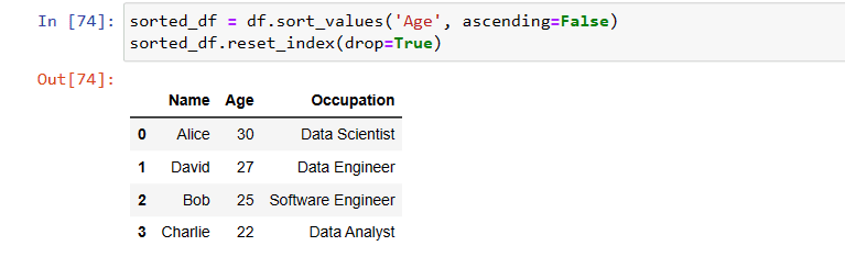

• reset_index is to use change the index values after sorting
• Parameter drop is used to drop the old index values

Pandas Dataframe Drop Rows with Condition

We can drop rows from pandas dataframe with condition. To drop rows in a Pandas DataFrame, we can use the DataFrame.drop() method. This method takes an index or a list of indices as an argument, and it drops the specified rows from the DataFrame.

#Drop the rows where the value in the column 'Name' is 'Bob'
df.drop(df[df.Name == 'Bob'].index, inplace=True)

OUTPUT
      Name  Age      Occupation
0    Alice   30  Data Scientist
2  Charlie   22    Data Analyst

#Drop the rows where the value in the column 'Name' is 'Bob'
df.drop(df[df.Name == 'Bob'].index, inplace=True)

OUTPUT
      Name  Age      Occupation
0    Alice   30  Data Scientist
2  Charlie   22    Data Analyst

Data Cleaning: Pandas Python Tutorial

Data cleaning is a pivotal aspect of data preparation, and Pandas offers an array of tools facilitating this process within Python. This vital stage involves cleaning, transforming, and refining raw data into a structured format suitable for analysis. Pandas empowers users to tackle common data wrangling challenges seamlessly.

Sorting Data

Sorting helps in arranging data for better insights.

df.sort_values("Price", ascending=False, inplace=True)

df.sort_values("Price", ascending=False, inplace=True)

Handling Missing Values:

Handling missing values is an essential part of data preprocessing. Pandas offers various methods to detect, handle, and manage missing data within DataFrames efficiently. Here are some common techniques to handle missing values:

Detecting Missing Values:

isnull() and notnull(): These methods return boolean masks indicating missing (True) or non-missing (False) values in the DataFrame or Series.

info(): Provides a summary of the DataFrame, showing the count of non-null values per column, which can help identify missing values.

Handling Missing Values:

fillna(): Replaces missing values with specified values like a constant, mean, median, or forward/backward fills. Let’s assume we have a pandas dataframe with few rows with no salary. We can replace it with any value using fillna() method.

df['Salary'].fillna(500, inplace=True)

df['Salary'].fillna(500, inplace=True)

dropna(): It removes rows or columns containing missing values based on specified thresholds (e.g., drop rows with any null value or only those with all null values).

df.dropna()

df.dropna()

Dealing with Duplicates:

df.drop_duplicates()

df.drop_duplicates()

Converting Data Types:

df['Salary'] = df['Salary'].astype(int)

Advanced Pandas Features

Grouping & Aggregation

Grouping helps in summarizing data based on specific categories.

grouped = df.groupby("Category")["Sales"].sum()

print(grouped)

grouped = df.groupby("Category")["Sales"].sum()

print(grouped)

Pivot Tables

Pivot tables help in restructuring and summarizing large datasets efficiently.

pivot = df.pivot_table(values="Sales", index="Category", columns="Region", aggfunc="sum")

print(pivot)

pivot = df.pivot_table(values="Sales", index="Category", columns="Region", aggfunc="sum")

print(pivot)

Merging & Joining DataFrames

Combining datasets is essential when working with multiple sources.

df1 = pd.DataFrame({"ID": [1, 2, 3], "Name": ["Amit", "Raj", "Suman"]})

df2 = pd.DataFrame({"ID": [1, 2, 3], "Salary": [50000, 60000, 70000]})

merged_df = pd.merge(df1, df2, on="ID")

print(merged_df)

df1 = pd.DataFrame({"ID": [1, 2, 3], "Name": ["Amit", "Raj", "Suman"]})

df2 = pd.DataFrame({"ID": [1, 2, 3], "Salary": [50000, 60000, 70000]})

merged_df = pd.merge(df1, df2, on="ID")

print(merged_df)

   ID   Name  Salary
0   1   Amit   50000
1   2    Raj   60000
2   3  Suman   70000

Data Visualization with 10 Minutes to Pandas

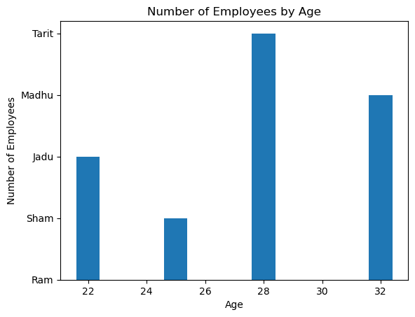
Basic plotting capabilities exist within Pandas for simple visualizations:

import pandas as pd
import matplotlib.pyplot as plt

# Create a DataFrame
df = pd.DataFrame({'Name': ['Ram', 'Sham', 'Jadu', 'Madhu', 'Tarit'], 'Age': [30, 25, 22, 32, 28]})

# Create a bar chart of the number of employees for each age
plt.bar(df['Age'], df['Name'])

# Add a title and labels
plt.title('Number of Employees by Age')
plt.xlabel('Age')
plt.ylabel('Number of Employees')

# Show the chart
plt.show()

import pandas as pd
import matplotlib.pyplot as plt

# Create a DataFrame
df = pd.DataFrame({'Name': ['Ram', 'Sham', 'Jadu', 'Madhu', 'Tarit'], 'Age': [30, 25, 22, 32, 28]})

# Create a bar chart of the number of employees for each age
plt.bar(df['Age'], df['Name'])

# Add a title and labels
plt.title('Number of Employees by Age')
plt.xlabel('Age')
plt.ylabel('Number of Employees')

# Show the chart
plt.show()

df['Age'].plot(kind='bar')

Advanced visualization can be achieved by integrating Pandas with libraries like Matplotlib and Seaborn.

Time Series Analysis in 10 Minutes to Pandas

Pandas excels in handling time series data:

dates = pd.to_datetime(['2020-01-01', '2020-02-01', '2020-03-01']) 
data = [10, 20, 30] 
time_series_df = pd.DataFrame({'Date': dates, 'Value': data})

dates = pd.to_datetime(['2020-01-01', '2020-02-01', '2020-03-01']) 
data = [10, 20, 30] 
time_series_df = pd.DataFrame({'Date': dates, 'Value': data})

  Date      	Value
0	2020-01-01	10
1	2020-02-01	20
2	2020-03-01	30

  Date      	Value
0	2020-01-01	10
1	2020-02-01	20
2	2020-03-01	30

With various time series operations like rolling averages, resampling, and trend analysis can be performed using Pandas’ functionalities we can easily use them for time series analysis.

Conclusion

In conclusion, this comprehensive guide covers essential 10 Minutes to Pandas Python Tutorial this includes functions, attributes, and operations, laying the groundwork for utilizing Pandas proficiently in data manipulation and analysis. You can also use PySpark to read very large CSV file more efficiently and quickly using Spark Distributed Architechure. You can review my earlier blog post to install PySpark in windows and how to read large CSV file using Python. I hope this article is useful. Please write in comment section if you have any questions, suggestions and ideas. Happy Coding!